Neural Architecture Search of Echocardiography View Classifiers
Project Introduction
Purpose
Echocardiography is the most commonly used modality for assessing the heart in clinical practice. In an echocardiographic exam, an ultrasound probe samples the heart from different orientations and positions, thereby creating different viewpoints for assessing the cardiac function. The determination of the probe viewpoint forms an essential step in automatic echocardiographic image analysis.
Approach
In this study, convolutional neural networks are used for the automated identification of 14 different anatomical echocardiographic views (larger than any previous study) in a dataset of 8,732 videos acquired from 374 patients. Differentiable architecture search approach was utilised to design small neural network architectures for rapid inference while maintaining high accuracy. The impact of the image quality and resolution, size of the training dataset, and number of echocardiographic view classes on the efficacy of the models were also investigated.
Results
In contrast to the deeper classification architectures, the proposed models had significantly lower number of trainable parameters (up to 99.9% reduction), achieved comparable classification performance (accuracy 88.4–96.0%, precision 87.8–95.2%, recall 87.1–95.1%) and real-time performance with inference time per image of 3.6–12.6 ms.
Conclusion
Compared with the standard classification neural network architectures, the proposed models are faster and achieve comparable classification performance. They also require less training data. Such models can be used for real-time detection of the standard views.
Dataset
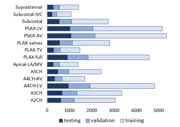
Fig. 1. Distribution of data in the training, validation and test dataset; values show the number of frames in a given class.
This project used the TTE47 dataset, developed from echocardiographic studies performed between 2010 and 2020 at Imperial College Healthcare NHS Trust.
For detailed dataset description, access request, and metadata, please refer to the dataset page below:
Request Access to TTE47 Dataset →
Network Architecture
DARTS Method
The DARTS method consists of two stages: architecture search and architecture evaluation.
Given the input images, it first embarks on an architecture search to explore for a computation cell (a small unit of convolutional layers) as the building block of the neural network architecture.
After the architecture search phase is complete and the optimal cell is obtained based on its validation performance, the final architecture could be formed from one cell or a sequential stack of cells. The weights of the optimal cell learned during the search stage are then discarded and reinitialised randomly for retraining the generated neural network model from scratch.
A cell is an ordered sequence of several nodes in which one or multiple edges meet. Each node C(i) represents a feature map in convolutional networks. Each edge (i,j) is associated with some operation O(i,j), transforming the node C(i) to C(j). This could be a combination of several operations, such as convolution, max-pooling, and ReLU. Each intermediate node C(i) is computed based on all of its predecessors.
Instead of applying a single operation (e.g., 5×5 convolution), and evaluating all possible operations independently (each trained from scratch), DARTS places all candidate operations on each edge (e.g., 5×5 convolution, 3×3 convolution, and max-pooling). This allows sharing and training their weights in a single process.
The actual operation at each edge is then a linear combination of all candidate operations O(i,j), weighted by the softmax output of the architecture parameters α(i,j).
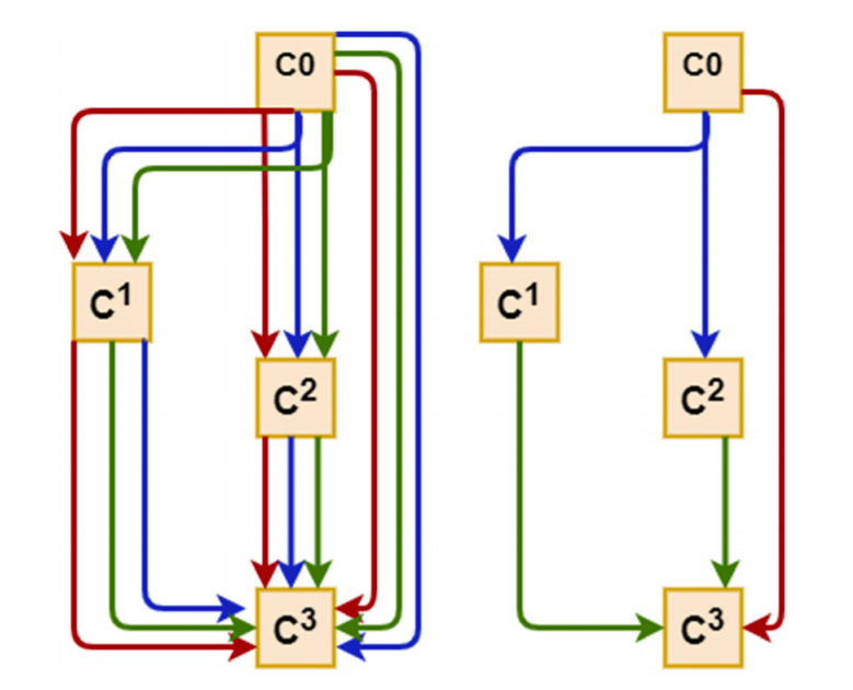
Fig. 2. Schematic of a DARTS cell.
Implementation
PyTorch was used to implement the models. For the computationally intensive stage of architecture search, a GPU server equipped with 4 NVIDIA TITAN RTX GPUs with 64 GB of memory was rented.
For the subsequent training of the searched networks and also the standard models, the utilised GPU was an Nvidia QUADRO M5000 with 8 GB of memory, representing a more widely accessible hardware for real-time applications.
Inference time (latency time for classifying each image) was also estimated with the trained models running on the GPU. To this end, a total of 100 images were processed in a loop, and the average time was recorded.
All training/prediction computations were carried using identical hardware and software resources, allowing for a fair comparison of computational time-efficiency between all network models investigated in this study.
The number of trainable parameters in the model, as well as the training time per epoch, was also recorded for all CNN networks.
Models Training Parameters
Training occurred subsequently, using annotations provided by the expert cardiologist. It was carried out independently for each of the four different image sizes of 32×32, 64×64, 96×96, and 128×128 pixels. Identical training, validation, and testing datasets were used in all network models.
The validation dataset was used for early stopping to avoid redundant training and overfitting. Each model was trained until the validation loss plateaued. The test dataset was used for performance assessment of the final trained models. The DARTS models were kept blind to the test dataset during the architecture search stage.
Adam optimiser with a learning rate of 1e−4 and a maximum of 800 epochs was used for training. The cross-entropy loss function was used as the network’s objective function.
The dataset is fairly imbalanced with unequal distribution of different echo views. To prevent potential biases towards dominant classes, online batch selection was used where an equal number of samples from each view were randomly drawn (by oversampling underrepresented classes).
This led to training on a balanced dataset representing all classes in every epoch.
Evaluation Metrics
Several metrics were employed to evaluate performance, including overall accuracy, macro average precision and recall, and the weighted F1 score (accounting for class imbalance).
Accuracy was computed as the fraction of correctly classified images, precision and recall averaged across views, and F1 score as the harmonic mean.
Results and Discussion
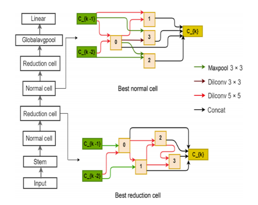
Fig. 3. Optimal normal and reduction cells for the input image size of 128×128 pixels.
Architecture Search
The search took approximately 6, 23, 42, and 92 hours for image sizes of 32×32, 64×64, 96×96, and 128×128 pixels respectively.
Two network architectures were assembled from the optimal cell: 1-cell-DARTS (single cell) and 2-cell-DARTS (stacked). Addition of more cells did not improve performance but increased redundancy.
| Input Size | Architecture | Accuracy (%) | Parameters (M) | Inference (ms) |
|---|---|---|---|---|
| 32×32 | 2-cell-DARTS | 93–96 | 0.5 | 3.6–7.2 |
| 128×128 | VGG16 / DenseNet201 | 88–94 | 5–100 | 10–12 |
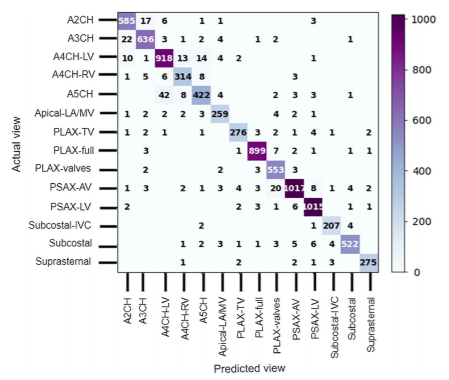
Fig. 4. Confusion matrix for the 2-cell-DARTS model (128×128 input).
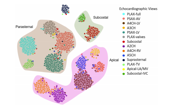
Fig. 5. t-SNE visualization of 14 echo views from the 2-cell-DARTS model.
Misclassifications were mainly between anatomically adjacent imaging planes, e.g., A4CH vs A5CH.
Even human experts disagree most often on these — highlighting inherent clinical ambiguity.
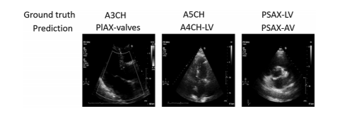
Fig. 6. Examples of misclassified cases.
Impact of Image Resolution, Quality, and Dataset Size
Models exhibited stable accuracy for image sizes ≥96×96 pixels. Smaller resolutions caused 2–5% performance drop, especially for fine structures (e.g., apical views).
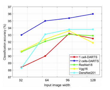
Fig. 7. Comparison of accuracy for different classification models and resolutions.
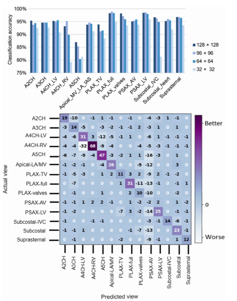
Fig. 8. Accuracy of 2-cell-DARTS model for various input image resolutions.
Larger image sizes offered only minor accuracy gains but higher compute cost.
Reducing training data affected deeper networks more than DARTS-based ones.
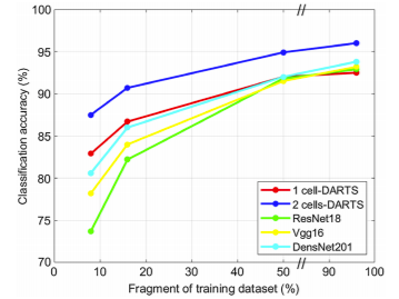
Fig. 9. Comparison of model accuracy across dataset sizes.
| Number of Echo Views | Accuracy (2-cell DARTS) |
|---|---|
| 14 views | 93% |
| 7 views | 97% |
| 5 views | 99.3% |
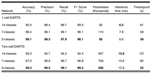
Table 2. Dependence of overall accuracy on number of echo views.
A correlation between image quality and accuracy was also observed.
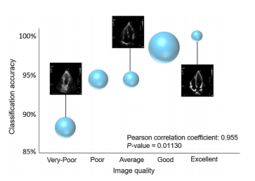
Fig. 10. Correlation between classification accuracy and image quality.